20200319_판다스(데이터 잔처리) - Jupyter Notebook.pdf
0.47MB
데이터 전처리
- 누락 데이터 처리
- 중복 데이터 처리
- 데이터 표준화
- 범주형 데이터 처리
- 정규화
- 시계열 데이터
누락 데이터 처리
20200319_판다스(데이터 잔처리).html
0.35MB
import seaborn as sns # seaborn 은 그래프화 해주는 라이브러리. 얘가 dataset을 제공을 해준다.
#titanic 데이터셋 가져오기
titanic_df = sns.load_dataset('titanic')
display(titanic_df.head())
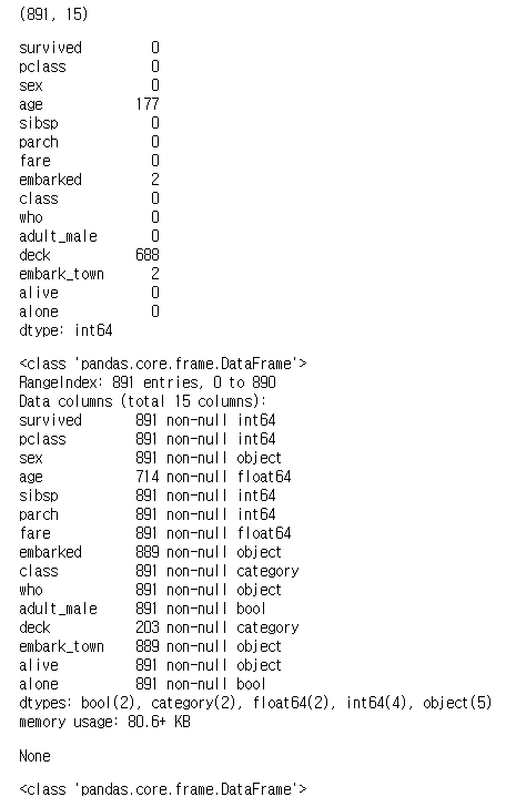
print(titanic_df.shape) # 891행, 15열
display(titanic_df.isnull().sum()) # null이 각각 몇개인지
display(titanic_df.info())
print(type(titanic_df))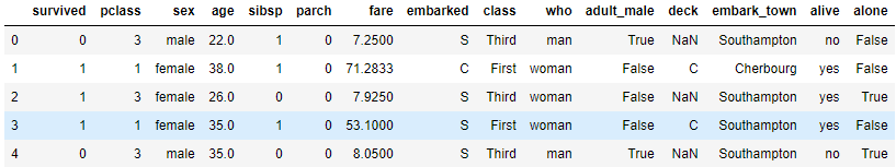
#value_counts
titanic_df.survived.value_counts()
0 549
1 342
Name: survived, dtype: int64
Q.deck 열의 NaN개수를 계산하세요.
#deck 열의 NaN 개수 계산하기
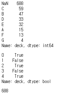
nan_deck = titanic_df['deck'].value_counts(dropna=False)
#nan_deck=df['deck'].value_counts()
print(nan_deck)
display(titanic_df['deck'].isnull().head())
print(titanic_df['deck'].isnull().sum(axis=0))#행방향으로 찾기
Q.titanic_df의 처음 5개 행에서 null값을 찾아 출력하세요(True/False)
# isnull()메소드로 누락데이터 찾기
display(titanic_df.head().isnull())
print()
display(titanic_df.head().notnull())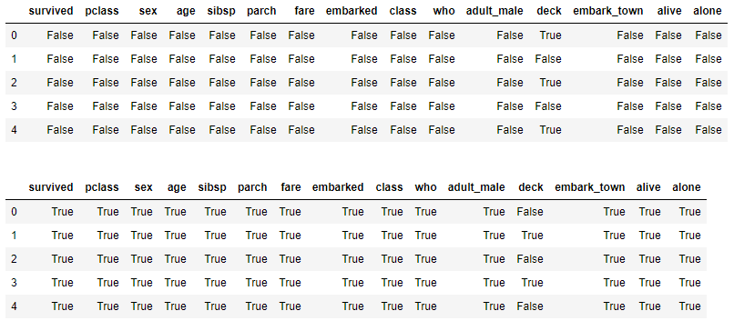
Q.titanic_df의 'deck' 칼럼의 null의 개수를 구하세요
# isnull()메소드로 누락데이터 개수 구하기
print(titanic_df.survived.isnull().sum(axis=0))
print(titanic_df.deck.isnull().sum(axis=0))
0
688
# 각 칼럼별 null 개수
print(titanic_df.isnull().sum(axis=0))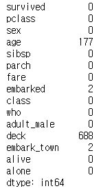
Q. titanic_df의 각 칼럼별 null의 개수를 for반복문을 사용해서 구한 후 출력하세요.
- (missing_count는 예외처리하고 처리 방식은 0을 출력함)
# thresh = 500: NaN값이 500개 이상인 열을 모두 삭제
#     - deck 열(891개 중 688개의 NaN 값)
# how = 'any' : NaN 값이 하나라도 있으면 삭제
# how = 'all':  모든 데이터가 NaN 값일 경우에만 삭제

df_thresh = titanic_df.dropna(axis=1, thresh=500)
# df1.dropna(axis=0) # NaN row 삭제
# df1.dropna(axis=1) # NaN column 삭제

print(df_thresh.columns)
Index(['survived', 'pclass', 'sex', 'age', 'sibsp', 'parch', 'fare', 'embarked', 'class', 'who', 'adult_male', 'embark_town', 'alive', 'alone'], dtype='object')
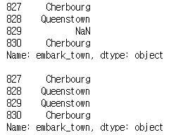
Q. embark_town 열의 NaN값을 바로 앞에 있는 828행의 값으로 변경한 후 출력하세요.
# embark_town 열의 NaN값을 바로 앞에 있는 828행의 값으로 변경하기
import seaborn as sns

titanic_df = sns.load_dataset('titanic')
titanic_df.embark_town.isnull().sum()
#print(titanic_df['embark_town'][827:831])
print(titanic_df.embark_town.iloc[827:831])
print()
titanic_df['embark_town'].fillna(method='ffill', inplace=True)
# Nan 데이터 0으로 채워줌
print(titanic_df['embark_town'][827:831])
중복 데이터 처리
# 중복데이터를 갖는 데이터 프레임 만들기
import pandas as pd
df = pd.DataFrame({'c1':['a','a','b','a','b'],
                  'c2':[1,1,1,2,2,],
                  'c3':[1,1,2,2,2]})
print(df)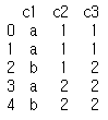
#데이터 프레임 전체 행 데이터 중에서 중복값 찾기
df_dup = df.duplicated()
print(df_dup)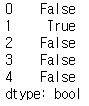
# 데이터프레임의 특정 열 데이터에서 중복값 찾기
col_dup_sum = df['c2'].duplicated().sum()
col_dup = df['c2'].duplicated()
print(col_dup_sum,'\n') # c2에서 중복되는 값이 몇개인지 확인
print(col_dup)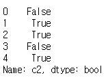
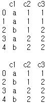
Q. df에서 중복행을 제거한 후 df2에 저장하고 출력하세요.
# 데이터 프레임에서 중복행 제거 : drop_duplicates()
print(df)
print()
df2= df.drop_duplicates()
print(df2)
Q. df에서 c2, c3열을 기준으로 중복행을 제거한 후 df3에 저장하고 출력하세요.
# print(df)
# print()
# df3= df[['c2','c3']].drop_duplicates()
# print(df3)

df3 = df.drop_duplicates(subset=['c2','c3'])
print(df3)
#[1,1] , [1,2],[2,2] 를 한묶음으로 봐서 같은 행을 삭제 한다.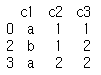
데이터 단위 변경
# read_csv() 함수로 df 생성
import pandas as pd
auto_df = pd.read_csv('auto-mpg.csv')
auto_df.head()
#mpg(mile per gallon)를 kpl(kilometer per liter)로 반환 (mmpg_to_kpl=0.425)
mpg_to_kpl = 1.60934/3.78541
print(mpg_to_kpl)
0.42514285110463595
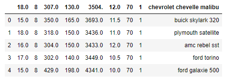
Q. 'mpg'를 'kpl'로 환산하여 새로운 열을 생성하고 처음 3개 행을 소수점 아래 둘째 자리에서 반올림하여 출력하시오.
import pandas as pd

# read_csv() 함수로 df 생성
auto_df = pd.read_csv('auto-mpg.csv', header=None)

# 열 이름을 지정
auto_df.columns = ['mpg','cylinders','displacement','horsepower','weight','acceleration','model year','origin','name']

display(auto_df.head(3))
print('\n')

auto_df['kpl'] = round((auto_df['mpg']*mpg_to_kpl),2)
display(auto_df.head(3))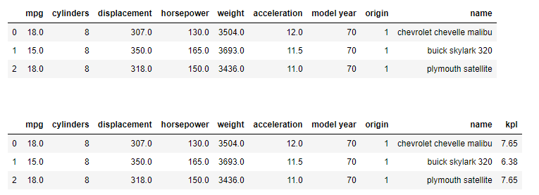
# 각 열의 자료형 확인
print(auto_df.dtypes)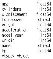
Q.horsepower 열의 고유값을 출력하세요.
print(auto_df['horsepower'].unique())
# '?' 때문에 horsepower       object로 모든 것을 인식한다.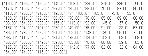
Q. horsepower 열의 누락 데이터 '?'을 삭제한 후 NaN 값의 개수를 출력하세요.
# 누락 데이터 ('?') 삭제
import numpy as np
auto_df['horsepower'].replace('?',np.nan,inplace=True) #'?'을 np.nan으로 변경
auto_df.dropna(subset=['horsepower'], axis=0, inplace=True) # 누락데이터 행을 제거
auto_df['horsepower'].isnull().sum()
print(auto_df.horsepower.dtypes)
object
Q. horsepower'문자열을 실수 형으로 변환 후 자료형을 확인하세요.
auto_dff=auto_df['horsepower'].astype('float')
print(auto_dff)
print(auto_dff.dtypes)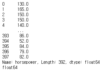
Q. 아래 사항을 처리하세요
# origin 열의 고유값 확인
print(auto_df['origin'].unique())

# 정수형 데이터를 문자형 데이터로 변환
auto_df['origin'].replace({1:'USA',2:'EU',3:'JAPEN'},inplace=True)

print(auto_df['origin'].unique())
[1 3 2]
['USA' 'JAPEN' 'EU']
origin 열의 자료형을 확인하고 범주형으로 변환하여 출력하세요.
# 연속형 (1,2,3,4,5..)/범주형('AG','BG'..)
print(auto_df['origin'].dtypes)
object
#origin 열의 문자열 자료형을 범주형으로 전환
auto_df['origin']=auto_df['origin'].astype('category')
print(auto_df['origin'].dtypes)
category
Q.origin열을 범주형에서 문자열로 변환한 후 자료형을 출력하세요
### origin 열의 자료형을 확인하고 문자형에서 범주형으로 변환하여 출력하세요.
auto_df['origin']=auto_df['origin'].astype('str') #str 대신 object를 사용 할 수 있다.
print(auto_df['origin'].dtypes)
object
Q.model year열의 정수형을 범주형으로 변환한 후 출력하세요
# auto_df['model year'].unique() : [70, 71, 72, 73, 74, 75, 76, 77, 78, 79, 80, 81, 82]
display(auto_df['model year'].sample(3))
auto_df['model year'] = auto_df['model year'].astype('category')
display(auto_df['model year'].sample(3))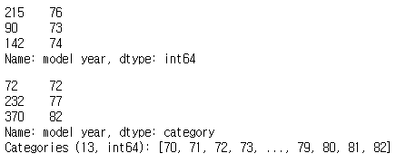
# 범주형(카테고리)데이터 처리
auto_df['horsepower'].replace('?',np.nan,inplace=True)
auto_df.dropna(subset=['horsepower'], axis=0, inplace=True)
auto_df['horsepower']=auto_df['horsepower'].astype('float')
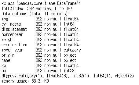
auto_df['hp']=auto_df['horsepower'].astype('int')
print()
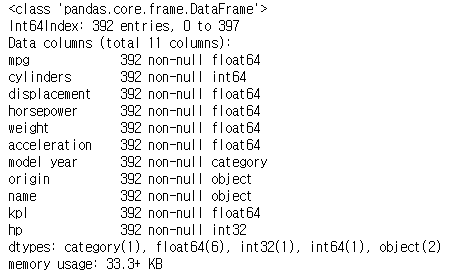
auto_df.info()
범주형(카테고리) 데이터 처리
auto_df['horsepower'].replace('?', np.nan, inplace=True)
auto_df.dropna(subset=['horsepower'], axis=0, inplace=True)
auto_df['horsepower'] = auto_df['horsepower'].astype('float')
auto_df['hp'] = auto_df['horsepower'].astype('int')
print()
auto_df.info()
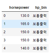
# np.histogram 함수로 3개의 bin으로 나누는 경계값의 리스트 구하기
count, bin_dividers = np.histogram(auto_df['horsepower'], bins=3) # 3개로 나누기 때문에 bins=3
display(bin_dividers) # [ 46. , 107.33333333, 168.66666667, 230.] : 46 ~ 107, 107 ~ 168, 168 ~ 230 총
print()

# 3개의 bin에 이름 지정
bin_names = ['저출력', '보통출력', '고출력']

# pd.cut 함수로 각 데이터를 3개의 bin에 할당
auto_df['hp_bin'] = pd.cut(x=auto_df['horsepower'],  # 데이터 배열
                           bins=bin_dividers,         # 경계 값 리스트
                           labels=bin_names,          # bin 이름
                           include_lowest=True)       # 첫 경계값 포함

# horsepower 열, hp_bin 열의 첫 5행을 출력
display(auto_df[['horsepower', 'hp_bin']].head())
array([ 46. , 107.33333333, 168.66666667, 230. ])
더미 변수
-카테고리를 나타내는 범주형 데이터를 회귀분석 등 ml알고리즘에 바로 사용할 수 없는 경우 -컴퓨터가 인식 가능한 입력값으로 변환 숫자 0 or 1로 표현된 더미 변수 사용. -0,1은 크고 작음과 상관없고 어떤 특성 여부만 표시(존재 1, 비존재 0) -> one hot encoding(one hot vector로 변환한다는 의미)
# hp_bin 열의 범주형 데이터를 더미 변수로 변환
horsepower_dummies = pd.get_dummies(auto_df['hp_bin'])
horsepower_dummies.head(15)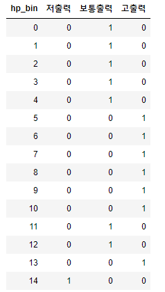
from sklearn import preprocessing

# 전처리를 위한 encoder 객체 만들기
label_encoder = preprocessing.LabelEncoder()        #label encoder 생성
onehot_encoder = preprocessing.OneHotEncoder()      #one hot encoder 생성

# label encoder로 문자열 범주를 숫자형 범주로 변환
onehot_labeled = label_encoder.fit_transform(auto_df['hp_bin'].head(15))
print(onehot_labeled)
print(type(onehot_labeled))
[1 1 1 1 1 0 0 0 0 0 0 1 1 0 2]
<class 'numpy.ndarray'>
# 2차원 행렬로 형태 변경
onehot_reshaped = onehot_labeled.reshape(len(onehot_labeled),1)
print(onehot_reshaped)
print(type(onehot_reshaped))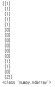
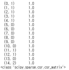
#희소행렬로 변환
onehot_fitted = onehot_encoder.fit_transform(onehot_reshaped)
print(onehot_fitted)
print(type(onehot_fitted))
정규화
- 각변수의 숫자 데이터의 상대적 크기 차이 때문에 ml분석결과가 달라질 수 있음.(a 변수 1 ~ 1000, b변수 0 ~ 1)
- 숫자 데이터의 상대적 크기 차이를 제거 할 필요가 있으며 각 열(변수)에 속하는 데이터 값을 동일한 크기 기분즈오 나누어 정교화 함
- 정규화 결과 데이터의 범위는 0~1 또는 -1 ~1(음수값이 있는 경우)
- 각열의 값/최대값 or (각 열의 값 - 최소값)/(해당 열의 최대값-최소값)표준화
- 평균이 0이고 분산(or표준편차)이 1인 가우시간 표준 정규분포를 가진 값으로 변환하는 것
- 표준화
- 평균이 0이고 분산(or표준편차)이 1인 가우시간 표준 정규분포를 가진 값으로 변환하는 것
# horsepower 열의 누락 데이터('?') 삭제하고 실수형으로 변환
auto_df = pd.read_csv('auto-mpg.csv', header=None)
auto_df.columns = ['mpg','cylinders','displacement','horsepower','weight','acceleration','model year','origin','name']
auto_df['horsepower'].replace('?', np.nan, inplace=True)      #'?'을 np.nan으로 변경
auto_df.dropna(subset=['horsepower'], axis=0, inplace=True)   # 누락데이터 행을 제거
auto_df['horsepower'] = auto_df['horsepower'].astype('float')  # 문자열을 실수형으로 변경

#horsepower 열의 통계 요약정보로 최대값(max)을 확인
print(auto_df.horsepower.describe())
print()

# horsepower 열의 최대값의 절대값으로 모든 데이터를 나눠서 저장

auto_df.horsepower = auto_df.horsepower / abs(auto_df.horsepower.max())

print(auto_df.horsepower.head())
print()
print(auto_df.horsepower.describe())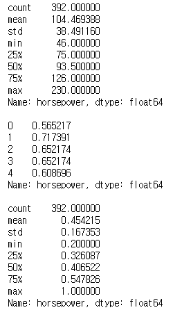
# read_csv() 함수로 df 생성
auto_df = pd.read_csv('auto-mpg.csv', header=None)
auto_df.columns = ['mpg','cylinders','displacement','horsepower','weight','acceleration','model yearr','origin','name']
#horsepower 열의 누락 데이터('?') 삭제하고 실수형으로 변환
auto_df['horsepower'].replace('?', np.nan, inplace=True)      #'?'을 np.nan으로 변경
auto_df.dropna(subset=['horsepower'], axis=0, inplace=True)   # 누락데이터 행을 제거
auto_df['horsepower'] = auto_df['horsepower'].astype('float') # 문자열을 실수형으로 변환

# horsepower 열의 통계 요약정보로 최대값 (max)과 최소값(min)을 확인
print(auto_df.horsepower.describe())
print()

# horsepower 각 열 데이터에서 해당 열의 최소값을 뺀 값을 분자, 해당 열의 최대값 - 최소값을 분모
# 가장 큰 값은 역시 1

min_x = auto_df.horsepower - auto_df.horsepower.min()
min_max = auto_df.horsepower.max() - auto_df.horsepower.min()
auto_df.horsepower = min_x / min_max

print(auto_df.horsepower.head())
print()
print(auto_df.horsepower.describe())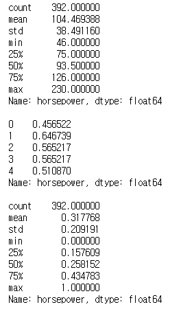
':: IT > python' 카테고리의 다른 글
| 20200316 python 판다스(pandas) 기초 (시리즈와 데이터프레임) (0) | 2020.03.20 |
|---|---|
| 20200320 python (전처리_시계열데이터) (0) | 2020.03.20 |
| 20200311 python (묘듈, 예외처리, 내장함수, map, 람다) (0) | 2020.03.19 |
| 20200310 python (함수, 사용자 입출력, 파일 읽고 쓰기, 클래스, 상속 ,오버라이딩, 오버로딩) (0) | 2020.03.19 |
| 20200308~20200309 python 기초 (0) | 2020.03.19 |